We’ve talked before about how to size bets and the interesting math behind it, the Kelly Critereon. A reasonable thought one might have after reading reading about Kelly is, “Gee, I have retirement investments, which are effectively bets on different stocks, bonds, and the like, and I would like to optimize my returns. What is the Kelly-optimal amount of money to allocate to each of these asset classes?”
Let me walk you through the math, but feel free to skip to the end if all you care about is the final answer. (Caveat: I’m not your investment advisor. Talk to them before doing anything with this information!!!)
The Kelly-optimal amount of money to allocate to a single investment is where f is the faction of your assets you should allocate to the investment, is the expected return of that asset, r is the risk-free rate of returns and is the standard deviation of the asset’s returns. Let’s do an example.
Let’s say you were thinking about buying US stocks. One reasonable way we could estimate expected returns is to look at what the stock market has returned on average in the past. A quick web search gave me the following return data I slapped in a spreadsheet to compute average and stdev:
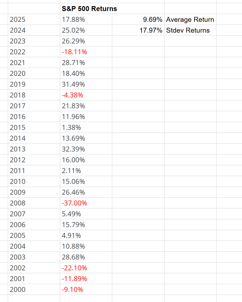
The mean of the returns, aka , is 9.7% and the standard deviation, , is 18%. You can adjust these predictions if you want – most analysts expect returns will be closer to 5.5% than 10% as an example – but I’ll just run with these numbers here. The last piece of data we need is the risk-free rate. If you’re new to this, the risk-free rate is just how much money you can earn with a completely risk-free asset. There’s some nuance around what exactly constitutes “risk-free”, but the 10-year US treasury rate, currently 4.1%, is a fine starting point.
Putting this altogether, Kelly says we should put , or 172% of my assets in the stock market.

What the math is saying is that this is such a good investment, the optimal strategy is to invest all of your money AND ALSO BORROW 72% MORE just to invest in stocks. Most people (myself included) would agree that this is totally nuts, so I’ll just pull out this quote from the previous article on Kelly
It’s also worth noting that strictly applying the Kelly formula often leads to very large bets that most people are uncomfortable with. In practice most people apply a multiplier (aka “fractional Kelly”) to reduce the exposure to wild swings in valuation
Alrighty, let’s do that. Most people use a fractional value between 1/2 (more aggressive) and 1/4 (less aggressive). Let’s use 1/3, which yields the fractional Kelly value of of our money in stocks. That seems plausible! But what do we do with the rest of our money? Let’s add some more asset classes to our portfolio. Similar to the S&P returns we can look up historic returns for whatever you want to invest in and you might end up with a chart like this:
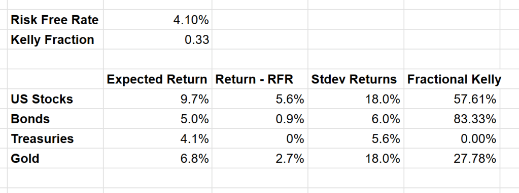
Ok… those fractional Kelly numbers add up to 168%, which again is the math telling us the optimal portfolio involves borrowing money. Most people aren’t into leverage, so you could just divide all the results by 1.68 to scale them down to a portfolio that adds up to 100%.
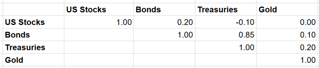
HOWEVER, these numbers ignore the very important fact that asset returns correlated. One of the reasons people invest in treasuries is that they tend to go up when stocks go down (and vice-versa), which helps make the overall portfolio more robust. So to compute the optimal portfolio we really need to know how correlated each asset is with the others.
If you have the yearly returns for each asset, you can calculate the the correlation coefficient directly (=CORREL() in Google Sheets), or just do another web search to find historical correlations. Doing so will give you a matrix like this:
Once we get correlations into the mix, there’s no longer a closed form solution to figuring out how much to invest in each asset. Instead we need to feed all this into an optimizer. Excel comes with one, but you can also use free ones, e.g., in python. At the bottom of this post is the code to compute our Kelly optimal portfolio with the constraints 1. no shorting any assets, 2. do not allocate more than 50% to any single asset, and 3. invest 100% of my money (no borrowing). If you don’t know how to run python, you can just paste the code in an online interpreter like here. When you run that it will spit out the optimal portfolio:
Risk-free baseline (Treasuries): 4.10%
Kelly fraction (fully invested): 0.33
Max position: 50.0%

Weights:
  Equities      :  44.86%
  IG Bonds      :  33.95%
  Treasuries    :   0.00%
  Gold          :  21.19%
There are a bunch of extensions you can make to get this slightly more realistic, but this great for most people. Please take the code, tweak the numbers, add assets, and see how the results compare to your current portfolio. Happy investing!
Update: if you found this interesting, I wrote some updates in a follow-on post.

import numpy as npfrom scipy.optimize import minimizedef build_cov_from_vol_corr(vol: np.ndarray, corr: np.ndarray) -> np.ndarray: vol = np.asarray(vol, float).reshape(-1) C = np.asarray(corr, float) n = vol.shape[0] if C.shape != (n, n): raise ValueError(f"corr must be shape ({n},{n}), got {C.shape}") C = 0.5 * (C + C.T) D = np.diag(vol) Sigma = D @ C @ D Sigma = 0.5 * (Sigma + Sigma.T) return Sigmadef fractional_kelly_constrained_scipy( assets: list[str], mu: np.ndarray, vol: np.ndarray, corr: np.ndarray, *, treasury_name: str = "Treasuries", kelly_fraction: float = 0.25, w_max: float = 0.40, # Mean uncertainty knobs effective_years: float = 5.0, uncertainty_aversion: float = 1.0, # Numerics ftol: float = 1e-12, maxiter: int = 50_000,) -> dict: """ Returns: dict with: w: optimal fractional-Kelly fully-invested weights (sum==1) rf: risk-free baseline (mu of Treasury) mu_excess: mu - rf Sigma: covariance matrix from vol/corr Sigma_mu: mean estimation covariance success/status: optimizer info diagnostics: objective components at solution """ if not (0.0 < kelly_fraction <= 1.0): raise ValueError("kelly_fraction must be in (0, 1].") if w_max <= 0: raise ValueError("w_max must be > 0.") if effective_years <= 0: raise ValueError("effective_years must be > 0.") if len(assets) == 0: raise ValueError("assets must be non-empty.") mu = np.asarray(mu, float).reshape(-1) vol = np.asarray(vol, float).reshape(-1) n = len(assets) if mu.shape[0] != n or vol.shape[0] != n: raise ValueError("assets, mu, and vol must have the same length.") if treasury_name not in assets: raise ValueError(f"treasury_name='{treasury_name}' not found in assets={assets}") treasury_idx = assets.index(treasury_name) Sigma = build_cov_from_vol_corr(vol, corr) # Treat Treasuries as risk-free baseline (excess return is zero for Treasuries) rf = float(mu[treasury_idx]) mu_e = mu - rf # "Grown-up" mean uncertainty: Sigma_mu = diag((vol/sqrt(T))^2) se = vol / np.sqrt(effective_years) Sigma_mu = np.diag(se**2) lam = float(uncertainty_aversion) # Fractional Kelly (fully invested) implemented by scaling the quadratic term by 1/f # Q is the effective quadratic form in the objective. Q = (Sigma + lam * Sigma_mu) / float(kelly_fraction) Q = 0.5 * (Q + Q.T) # ensure symmetry # We maximize: mu_e^T w - 0.5 w^T Q w # SciPy minimizes, so minimize negative: def obj(w: np.ndarray) -> float: w = np.asarray(w, float) return -(mu_e @ w - 0.5 * (w @ (Q @ w))) def grad(w: np.ndarray) -> np.ndarray: w = np.asarray(w, float) # d/dw [-(mu_e^T w - 0.5 w^T Q w)] = -mu_e + Q w return -mu_e + Q @ w # Fully invested: sum(w) == 1 cons = [{ "type": "eq", "fun": lambda w: np.sum(w) - 1.0, "jac": lambda w: np.ones_like(w), }] # Long-only + max position bounds = [(0.0, float(w_max)) for _ in range(n)] # Feasible initialization: equal weight, then project to bounds and renormalize w0 = np.full(n, 1.0 / n) w0 = np.clip(w0, 0.0, w_max) s0 = w0.sum() if s0 <= 0: w0[treasury_idx] = 1.0 else: w0 = w0 / s0 # satisfy sum==1 # If w_max < 1/n, equal-weight init will violate sum==1 after clipping; fix by packing. if (1.0 / n) > w_max: # Greedy pack: allocate w_max from start, remainder to treasury w0 = np.zeros(n) rem = 1.0 for i in range(n): take = min(w_max, rem) w0[i] = take rem -= take if rem <= 1e-12: break # If still remainder because all hit w_max, infeasible unless n*w_max >= 1 if rem > 1e-10: raise ValueError(f"Infeasible: n*w_max={n*w_max:.3f} < 1. Increase w_max or number of assets.") res = minimize( obj, w0, method="SLSQP", jac=grad, bounds=bounds, constraints=cons, options={"ftol": ftol, "maxiter": maxiter, "disp": False}, ) if not res.success: raise RuntimeError(f"Optimization failed: {res.message}") w = np.clip(res.x, 0.0, w_max) # Numerical cleanup to ensure exact sum==1 (SLSQP is close but not perfect) # Simple renormalization within bounds; if it breaks bounds, we do a bounded projection step. def project_to_simplex_with_bounds(w_in: np.ndarray, lo: float, hi: float, target_sum: float = 1.0) -> np.ndarray: """ Project onto {w: sum(w)=target_sum, lo<=w<=hi} using bisection on Lagrange multiplier. """ w_in = np.asarray(w_in, float) # We solve: w = clip(w_in - t, lo, hi) with sum(w)=target_sum # Monotone in t => bisection. t_lo, t_hi = -1e6, 1e6 for _ in range(200): t_mid = 0.5 * (t_lo + t_hi) w_mid = np.clip(w_in - t_mid, lo, hi) s = w_mid.sum() if abs(s - target_sum) < 1e-12: return w_mid if s > target_sum: t_lo = t_mid else: t_hi = t_mid return np.clip(w_in - 0.5 * (t_lo + t_hi), lo, hi) w = project_to_simplex_with_bounds(w, 0.0, w_max, 1.0) return { "assets": assets, "w": w, "rf": rf, "mu": mu, "mu_excess": mu_e, "vol": vol, "Sigma": Sigma, "Sigma_mu": Sigma_mu, "kelly_fraction": kelly_fraction, "w_max": w_max, "effective_years": effective_years, "uncertainty_aversion": lam, "success": bool(res.success), "status": res.message, }if __name__ == "__main__": assets = ["Equities", "IG Bonds", "Treasuries", "Gold"] mu = np.array([0.097, 0.05, 0.041, 0.068]) vol = np.array([0.18, 0.06, 0.056, 0.18]) corr = np.array([ [ 1.0, 0.2, -0.1, 0.0], [ 0.2, 1.0, 0.85, 0.1], [-0.1, 0.85, 1.0, 0.2], [ 0.0, 0.1, 0.2, 1.0], ]) out = fractional_kelly_constrained_scipy( assets=assets, mu=mu, vol=vol, corr=corr, treasury_name="Treasuries", kelly_fraction=0.33, # 1/3 Kelly w_max=0.50, # max position constraint effective_years=5.0, # mean estimate confidence uncertainty_aversion=1.0, # how skeptical you are of means ) print(f"Risk-free baseline (Treasuries): {100*out['rf']:.2f}%") print(f"Kelly fraction (fully invested): {out['kelly_fraction']:.2f}") print(f"Max position: {100*out['w_max']:.1f}%\n") print("Weights:") for a, w in zip(out["assets"], out["w"]): print(f" {a:14s}: {100*w:6.2f}%")

Leave a comment